


Abstract
High crime rate in the United States, although having been mitigated substantially since the late 2000s, is recurring in the past ten years. In particular, homicide rate in the US is extremely high compared with that in the EU countries. And the vicious crime cycle potentially caused by malfunctions of disadvantaged community would crack the social orders and exacerbate inequality. While classic studies tend to perceive communities as static (Airaksinen et al., 2021), recent trends prefer dynamic thinking (Levy et al., 2021). Criminal activities could diffuse within communities, spread across neighborhood, and even transmit beyond neighborhood.
This study applies Network Analysis (NA) to track the relationship between community mobility and crime rates with Big Data from New York TLC Trip Record. Both the Linear regression model and the Exponential Random Graph Model (ERGM) are selected to study interrelations between community mobility and crime rates. Results from the first approach confirms crime patterns that are beyond adjacent neighborhoods. Related effects are determined by the degree of crime-centered (the Top 3). As ranking of crime rate decreased, the impacts shrunk as well. In general, given other factors constant, inflows of people from crime-centered areas are correlated with higher crime rates, and vice versa.
Using a subset of the data (the weight threshold set above 1000 times), the second approach indicated the mutuality of the ties of travel; besides, the connection between area-centered in general sense are strong and poverty-stricken areas tend to connect with areas with similar attributes. The formation of crimes and their diffusion could be more sophisticated. While results from our models confirm previous assumptions, this study might be further enhanced by considering relationship between taxi and other modes of transportation, using a more consistent data merging approach, and reconstructing methods to separate the effects of neighborhood in crime distribution.
Part I Introduction
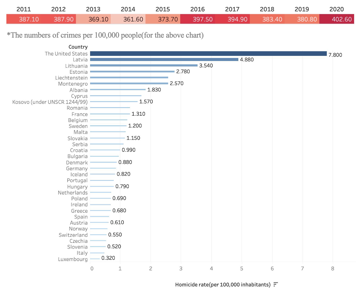
The United States has a relatively high crime rate among developed economics; even though the number has decreased significantly since the late 20th century, the high crime rate is still recurring in recent years (see Figure 1). What’s more, the country continues to grapple with a range of criminal activities, while homicide is on the top. In 2020, the homicide rate in the US was 7.8, almost double the worst situation in the EU countries and even more than 24 times Luxembourg’s data. This could be largely attributed to the country’s socially permissive attitude towards firearms.
Besides, crimes are likely to cluster around specific communities, such as immigrant and minority neighborhoods in cities with great diversity like New York. Such crime pattern highlights the correlation between racial segregation and crime rate, which could be caused by the enormous gaps in socio-economic status (Harrison & Beck, 2002). Violence might be an option to achieve some unjust goals (Black, 1983), and data imply that people with lower socio-economic status tend to have stronger motivations to adopt coercion to resolve conflicts (Anderson, 2000). This is because violence may sometimes operate as a subculture, by which the minority groups adapting to adverse environments expressed dissatisfaction and retaliated through physical fights.
Malfunctions of some communities, in particular, the disadvantageous ones, can exacerbate criminal activities. While community is perceived as a geographic unit that can facilitate internal cohesion through neighborhood ties, it does not respond to crimes effectively due to “opportunity structures”. The wealthier communities are more likely to organize collective actions to combat crime, while disadvantaged communities could not address the issues adequately. Others have found that criminal behaviors can spread spatially (Peterson & Krivo, 2010; Cohen & Tita, 1999; Morenoff et al., 2001; Sampson, 2012).
The most recent trends have found crime patterns that are beyond neighborhood using computational approaches. This project utilizes big data from New York TLC Trip Record to demonstrate urban mobility. Based on Network Analysis, this study extends the scope of crime identification.
Part II Literature Review
The determinants for criminal activities have been intensively explored; and among the studies, the role of communities and functions of neighborhood are the ones frequently highlighted. Classic research on violence and crimes emphasizes socioeconomic status of the perpetrators. At the aggregated level as communities, different neighborhood effects on the social order emerge. Related studies working on the effect of the neighborhood on crime have shifted from explaining the internal causes to identifying external interactions among communities that catalyze crime.
A. Within Residential Community: A Traditional Approach
There are mainly three perspectives explaining causes of community crime, including social disorganization, routine activities, and structural culture. Social disorganization proposes that the ecological conditions of community manifested as inferior SES, high racial heterogeneity, and frequent replacement of residents exert a negative influence on social ties and provide soil for deviant behaviors (Shaw & McKay 1942; Bursik & Grasmick, 2001). The concept of community efficacy was raised, indicating that people living together can gradually form social cohesion and establish voluntary supervision of negative behavior (Sampson et al. 1997). The place-based theory assumes that time and space interaction of people influence the occurrence of crime, where a motivated offender, a suitable target, and the absence of guardian coexist (Cohen & Felson 1979). Cultural theory focuses on structural factors, underlining that a culture of violence results in more crime within the neighborhood (Merton, 1938).
However, all these prioritize inherent cohesion of a community but ignore that action scripts of individuals can vary under different community backdrops. Empirical works have turned to collect meso and macro characteristics of communities of crime. Among them, reference to National surveys is most common. Other data sources include self-collected investigations and artificial rating segments (Massey et al., 1989; Sampson 1999). In a more recent attempt, survey data is selected to distinguish the sequential mechanisms of informal control and network in combating community crimes (Bellair et al., 2010).
B. Cross Boundaries of Neighborhoods: A New Measurement
Studies have provided evidence that crime does not necessarily concentrate only within independent communities but can also spread between connected neighborhoods. Economic status of neighboring communities is found to be an effective predictor of violence (Krivo, 2010). Diffusion of crimes could cross the boundary of neighborhoods (Cohen and Tita, 1999; Morenoff et al., 2001; Sampson, 2012), as evidenced by individual acts of co-offending spreading among Chicago neighborhoods spatially (Papachristos & Bastomski, 2018). The sprawling feature of crime inspires studies to treat communities as surroundings of individual residence, instead of administrative boundaries (Hipp & Boessen, 2013).
The intersection of mobility and crime pattern gradually attracts more academic attention. Non-residential neighborhoods provide exposure to different resources, information and institutions and could enhance the possibility of crime involvement (Graif et al., 2021). Research found that people spend more than half of their time outside their hometowns, and those with high criminal inclination are more likely to spend more time hanging out (Wikström et al., 2010). Big data has become conducive in identifying the distribution and changing trajectory of criminal events. Density of community-insider Twitter users and their tweets (Vomfell et al., 2018; Levy et al., 2020; Wo et al., 2022), anonymized dataset from Foursquare (Kadar et al., 2020) and taxi records (Wang et al., 2016) show accuracy in predicting where crime will occur.
This research uses taxi travel record data that are more tidy, straightforward, and representative. Potential contribution is twofold: using large-scale data can more accurately characterize community mobility from the perspective of traffic travel; and this research could contribute to crime identification strategies by establishing an integrated model incorporating travel data, crime rate and poverty rate.
Part III Research Design and Methodology
This research aims to use taxi record data to represent part of the mobility pattern within New York City, linked with the distribution of crime by locations. Research questions are: What’s the correlation between urban mobility and distribution of crimes in New York? What are the possible interpretations for the identified correlation? The key hypothesis is that predefined crime-centered regions tend to connect with similar areas through urban mobility, even when those connections are beyond adjacent neighborhoods.
The basic research idea is built upon Network Analysis (NA). By pairing pickup and drop-off points of taxi records, the physical mobility of each travel is drawn as a graph G = (V, E), where V refers to nodes (locations) and E demonstrates the linkage between them. It is a directed network. External factors are introduced to establish assumed linkages with the travel network, verified first by linear regression, then by Exponential Random Graph Model (ERGM).
For the first approach, edge weight summarizes the frequency of taxi transportation (with direction). The inflow and outflow of passengers from crime-centered areas serve as independent variables, while crime rate serves as the dependent variable. For ERGM, attributes of nodes include population, crime rate, and socio-economic aspects. The edge is modified by edge weight to demonstrate the strength of ties. The model is evaluated by AIC and BIC.
Part IV Research Data, Results, and Analysis
A. Overview of Key Datasets
There are two main datasets: the TLC Trip Record Data with physical mobility of passengers and the NYPD Complaint Data with crime distribution. One challenge is the inconsistency in classifying variables. The taxi records are labelled by taxi zone, which is not compatible with the geographic information traditionally used for categorizing socio-economic status (SES). We have reclassified travel records by police precinct, with classification determined based on the dominant area. For population data at precinct level, we used a transformed 2020 census data created by Keefe (2022). Other related factors, such as SES, are obtained from the US Census Data with certain transformation.
| TLC Trip Record Data | NYPD Complaint Data | |
|---|---|---|
| Content | Travel records by taxi zone | General crime records by precinct |
| Source | Taxi & Limousine Commission | New York City Police Department |
| Description | Update monthly from 2009/01 | Update quarterly from 2000/01 |
| Variable | Pickup and drop-off locations, and time of travel records, etc. | Address of the complained crime, and occurring time of crimes, etc. |
| Format | PARQUET | CSV |
TLC trip records are available at: https://www.nyc.gov/site/tlc/about/tlc-trip-record-data.page; and crime data at: https://www.nyc.gov/site/nypd/stats/stats.page.
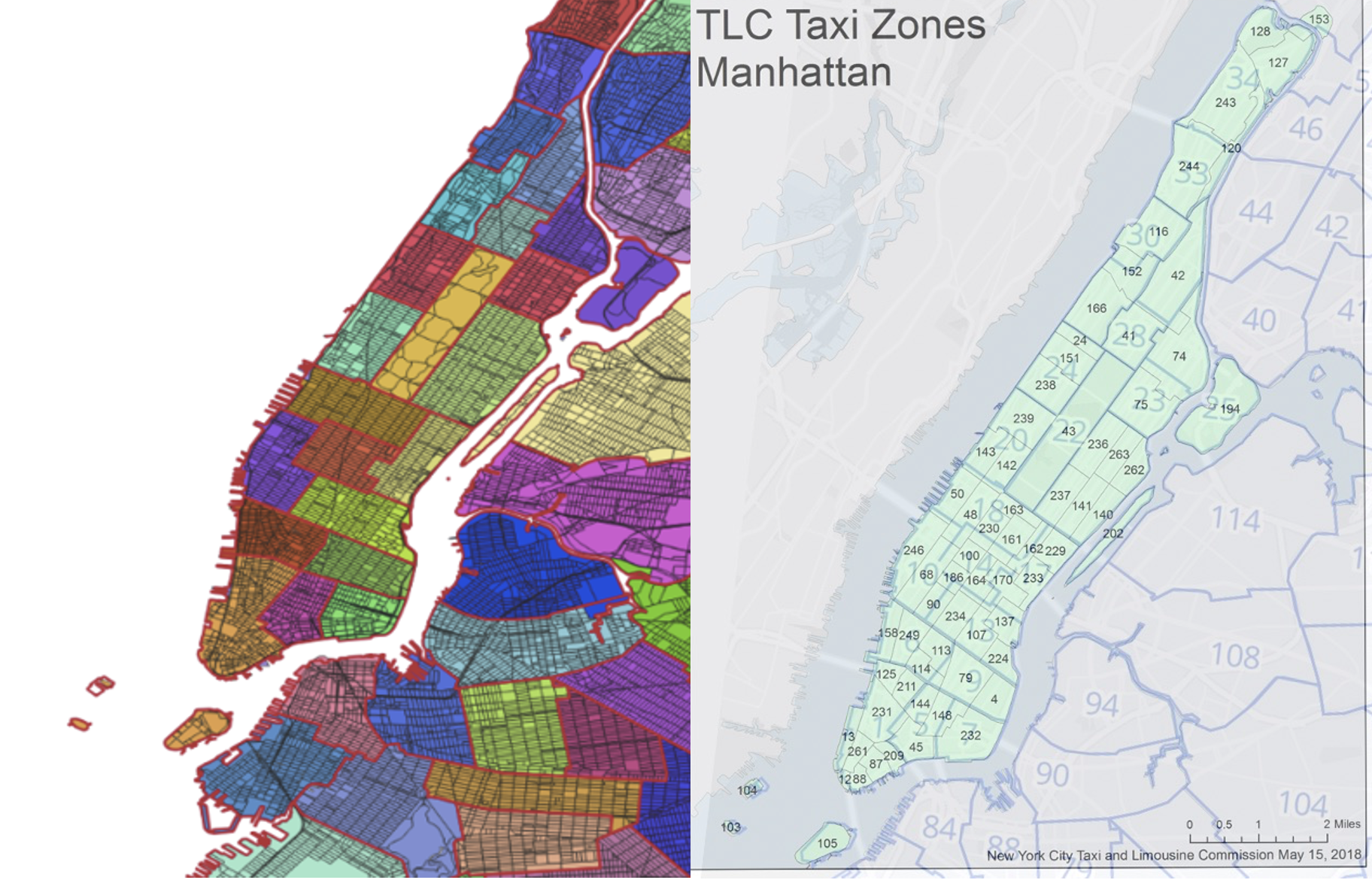
Picture on the left is available at https://johnkeefe.net/nyc-police-precinct-and-census-data. Picture on the right is the combination of two shapefiles from New York TCL and Open Data Portal.
Concatenating the yellow taxi driving records in 2020, we have obtained around 40 M (39,656,098) pairs of data. A directed network has been created using both pickup and drop-off locations. The travel path with the same departure and destination are summed up as the edge weights to measure the strength of ties (from the perspective of mobility) between two precincts. This step has simplified the network as a framework containing 6,074 rows, representing the 6,074 kinds of directions between travel areas.
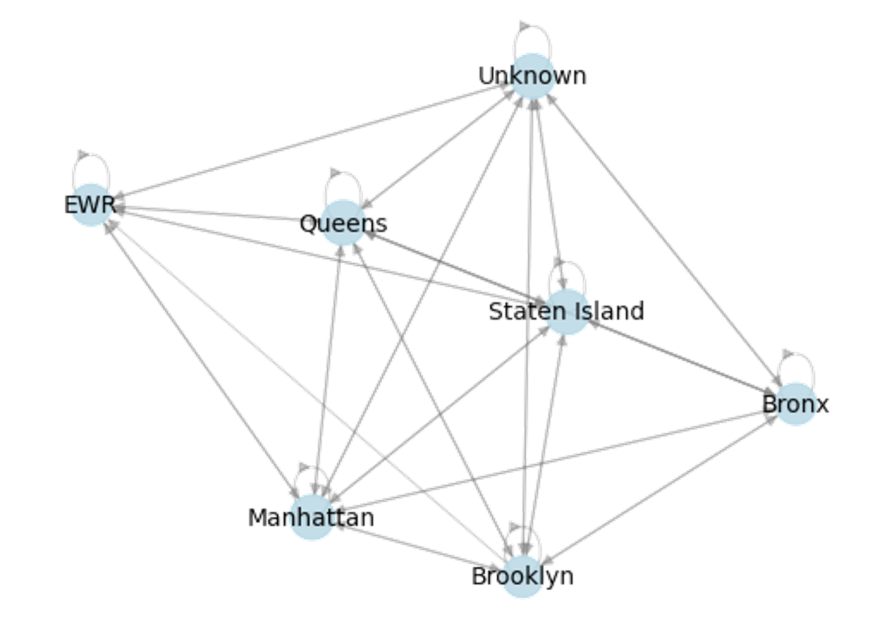
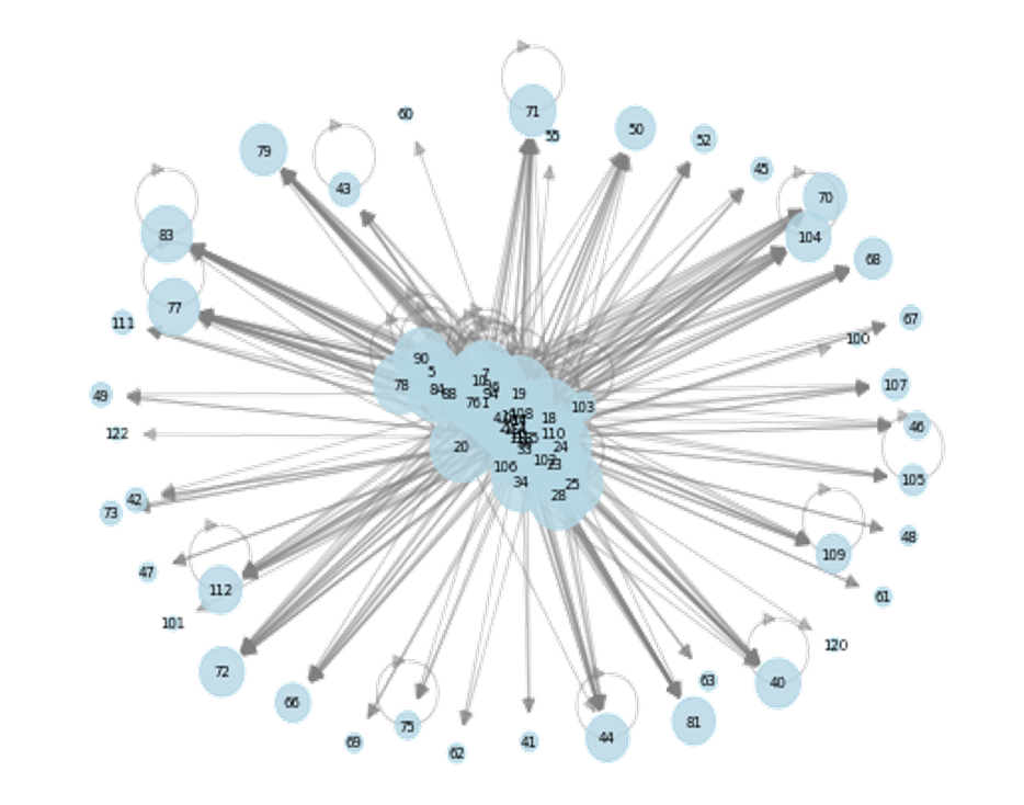
The following graphs have presented features of the travel network in a straightforward way. At Borough level, all areas seem to be interconnected, and self-loops are common. At the micro level, a considerable share of the precincts connected with one another via taxi travel. However, different from the Borough level data, precinct level data are more heterogeneous with some only having self-loops and being isolated (i.e., No. 43 Precinct).
B. Linear Regression Models
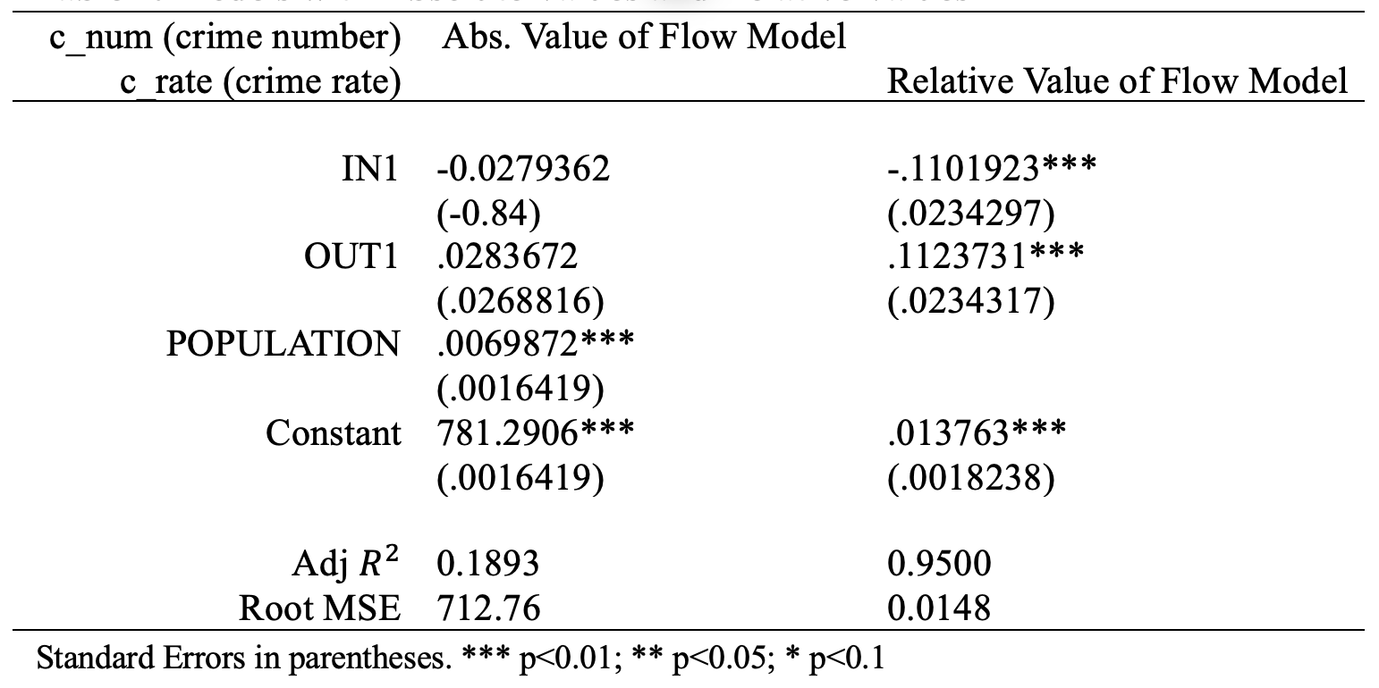
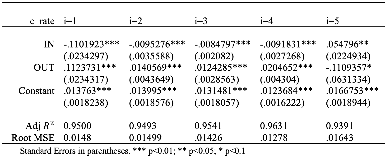
First of all, we selected two functional forms of the data, using either the absolute values or relative values. The results imply that relative values measure the crime distribution better (see Table 2; results are similar when the value of k changes and just k=1 is shown). When inflows of passengers from the most crime-centered area, a 1% increase (in relation to population base in the destination), would decrease crime rate by about 11.02%; the outflows, through a similar channel, would increase crime rate by around 11.24%. The effects of inflows when k=2, 3 are 0.95% and 0.85% with same signs, while of outflows, are 1.41% and 1.24% respectively. Starting from k=4, either the absolute values or the signs of coefficient change.
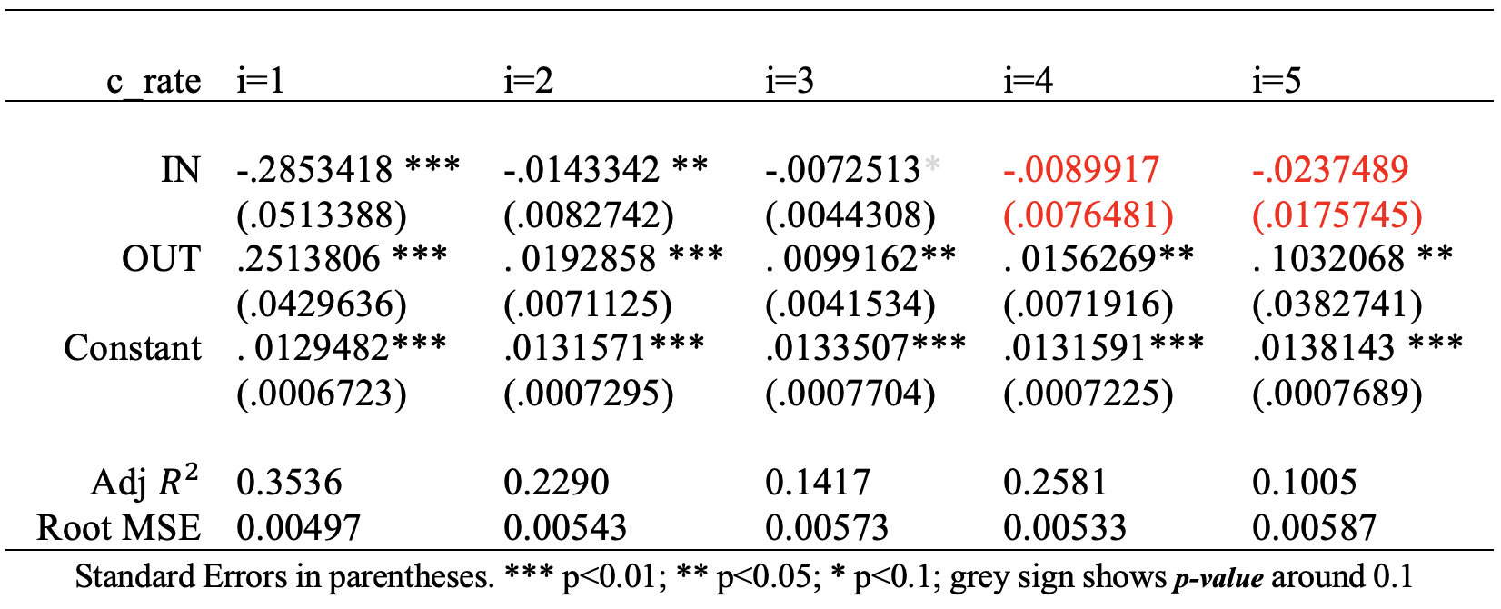
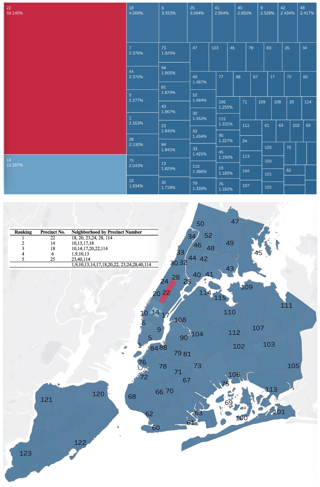
The second attempt for linear modeling excludes precincts that are right next to crime-centered areas (see Figure 4 and Table 4). The model yields the same outcome patterns, and even higher coefficients in the sake of substantially lower Adj R² value. But starting from k=4, impacts of inflow were not statistically significant.
C. Exponential Random Graph Model (ERGM)
After basic linear regression, we have also tried ERGM for statistical network modeling. The ERGM enables attributes to be added in the network at the micro levels. The model is often employed using R Studio. However, restricted by the capacity of the software, which can read 50,000 rows of data at one time, our original datasets cannot feed into the software altogether. We chose to compress the original networks using weight of travel.
First of all, the model is used to specify a single homogeneous probability for all ties, as captured by the coefficient of edge. The log-odds that a tie for the edges term equals to one for all pairs is presented as: logit(p) = exp(1.97572) / (1 + exp(1.97572)) = 0.8782242, which is corresponding to the density of the entire network.
| Estimate | Std. Error | MCMC% | z value | Pr(>|z|) | |
|---|---|---|---|---|---|
| Maximum Likelihood Results (Entire Network, Edges Only) | |||||
| edges | 1.97572 | 0.03871 | 0 | 51.05 | <1e-04 *** |
| Null Deviance: 8652 on 6241 DoF, Residual Deviance: 4624 on 6240 DoF | |||||
| AIC: 4626 BIC: 4633 | |||||
| Monte Carlo Maximum Likelihood Results (Entire Network) | |||||
| edges | 1.2897 | 0.1217 | 0 | 10.596 | <1e-04 *** |
| mutual | 0.9374 | 0.1424 | 0 | 6.584 | <1e-04 *** |
| Null Deviance: 8652 on 6241 DoF, Residual Deviance: 4581 on 6239 DoF | |||||
| AIC: 4585 BIC: 4598 (MC Std. Err. = 0.7574) |
Significant codes: 0 '***' 0.001 '**' 0.01 '*' 0.05 '.' 0.1 ' ' 1
| Estimate | Std. Error | MCMC% | z value | Pr(>|z|) | |
|---|---|---|---|---|---|
| Maximum Likelihood Results (Network Subset, Edges Only) | |||||
| edges | -1.86821 | 0.03815 | 0 | -48.97 | <1e-04 *** |
| Null Deviance: 8219 on 5929 DoF, Residual Deviance: 4666 on 5928 DoF | |||||
| AIC: 4668 BIC: 4674 | |||||
| Monte Carlo Maximum Likelihood Results (Trimmed Network) | |||||
| edges | -2.5502 | 0.0565 | 0 | -45.14 | <1e-04 *** |
| mutual | 2.7074 | 0.13090 | 2 | 20.68 | <1e-04 *** |
| Null Deviance: 8219 on 5929 DoF, Residual Deviance: 4198 on 5927 DoF | |||||
| AIC: 4202 BIC: 4215 (MC Std. Err. = 1.942) |
Significant codes: 0 '***' 0.001 '**' 0.01 '*' 0.05 '.' 0.1 ' ' 1
Monte Carlo Maximum Likelihood Results in Table 5 indicate that there is a statistically significant mutuality effect. Conditional log-odds of two places constructing a tie are: 1.2897 x change in the number of ties + 0.9374 x change in number of mutual dyad. If adding a tie would not make a reciprocal, its log-odds = 1.2897; if it would, its log-odds = 2.2271. The corresponding probabilities for them are 0.7841 and 0.9027 respectively.
To reduce calculating errors caused by treating all the ties indiscriminately, original data has been further trimmed and only the edge weight above 1000 has been retained. The operation generates log-odds at -1.86821, a statistical equivalent of 0.13375 probability. Although the mutuality effect is still statistically significant, coefficients for the two items are very close (-2.55 for edges, and 2.71 for mutual). Apart from crime rate previously utilized, we also introduce another new variable as the node attribute, namely, the poverty rate.
| Estimate | Std. Error | MCMC% | z value | Pr(>|z|) | |
|---|---|---|---|---|---|
| edges | 1.8615 | 0.2253 | 0 | 8.261 | <1e-04 *** |
| nodecov.povertyrate | -5.0334 | 0.4623 | 0 | -10.887 | <1e-04 *** |
| nodecov.crimerate | -58.5968 | 4.4538 | 0 | -13.157 | <1e-04 *** |
| Null Deviance: 8219 on 5929 DoF; Residual Deviance: 4352 on 5926 DoF | |||||
| AIC: 4358 BIC: 4378 (MC Std. Err. = 0) |
Significant codes: 0 '***' 0.001 '**' 0.01 '*' 0.05 '.' 0.1 ' ' 1
| Estimate | Std. Error | MCMC% | z value | Pr(>|z|) | |
|---|---|---|---|---|---|
| edges | -1.38844 | 0.05976 | 0 | -23.232 | <1e-04 *** |
| absdiff.povertyrate | -4.86980 | 0.57949 | 0 | -8.404 | <1e-04 *** |
| absdiff.crimerate | -28.37234 | 5.61123 | 0 | -5.056 | <1e-04 *** |
| Null Deviance: 8219 on 5929 DoF; Residual Deviance: 4538 on 5926 DoF | |||||
| AIC: 4544 BIC: 4564 (MC Std. Err. = 0) |
Significant codes: 0 '***' 0.001 '**' 0.01 '*' 0.05 '.' 0.1 ' ' 1
Results in Table 7 imply that both poverty rate and crime rate are statistically significant for the formation of a link, with the negative impacts from crime being more prominent. Higher crime rates might deter travel to the crime-centered areas, and thus the linkage between any given place and the targeted location would be difficult to establish. In the model shown in Table 8, where the Absdiff function has been applied, similar outcomes emerge. The function is adopted to test whether nodes with similar level attributes tend to connect with each other. Our results confirm this trend, and crime plays a greater role.
Part V Conclusion, Research Limitation, and Further Studies
As indicated by the results in the previous sections, certain relationship exists between urban mobility and the distribution of crime in New York. Although formation of crimes could be structural and sophisticated, the spatial diffusion of people either coming from or travelling to the crime-centered areas could play a role. But to be defined as a crime-centered area, the standard could be rather strict; in our case, areas with the Top 3 crime rate would satisfy the criteria, as they always have statistically significant influence on crime rates in connected areas.
Incorporating all areas of interest, the linear regression model has demonstrated great predictive powers, as the Adj R² are always around 0.95. The inflows of people from the crime-centered areas by taxi, surprisingly decreased the crime rate of the local region. By contrast, the outflow of people to the crime-centered areas increased the crime rate in the pickup areas. Besides, the power of these influences decreases as the severity of crime of targeted areas decline. Also, we have excluded areas around crime-centered communities to explore spatial influences that are potentially beyond adjacent neighborhoods. Our models show that conclusions from the full dataset could still apply, although the Adj R² have decreased substantially.
Reasons for the signs of coefficient might be explained by: (1) taxi users are normally with better SES, and even inflows from the crime-centered areas are good citizens bringing positive impacts; (2) travel to crime-centered areas might expose to or receive negative impacts, which then exercised its effects at home; (3) the larger proportion of taxi passengers implies a smaller share of people travelling by public transportation, given the total fixed. The ERGM has contributed by demonstrating structure of communities as well as implying the interconnectivity of regions with similar attributes.
Although this research has tried to be as rigorous as possible, it still suffers from several limitations. The first aspect relates to our research data. Taxi travel, although being an essential part of the regional transportation, could be biasedly selected. Yellow taxi is only part of the taxi market, and its representativeness of the whole industry requires further verification. In addition, the cost for taxi travel would be high and passengers choosing this mode may possess better socio-economic status. The second aspect relates to our reclassification of the data. Disaggregation might cause greater errors in the process of transformation. The third aspect is the treatment of the neighborhood. Although the study has attempted to separate effects of neighborhood by removing those around the crime-centered areas, interactions among the communities are much more complicated.
For further studies, the representativeness of yellow taxi of the entire industry could be considered and verified (or just include all types of taxi data as the research subjects). Besides, the interrelation of taxi with other modes of transportation, such as bus, subways, and self-drive could be established for a more accurate interpretation of research results.